[Improving: Hyper-parameter tuning, Regularization and Optimization] Programming - Regularization

This note is based on Coursera course by Andrew ng.

(It is just study note for me. It could be copied or awkward sometimes for sentence anything, because i am not native. But, i want to learn Deep Learning on English. So, everything will be bettter and better :))

 

 

 

INTRO

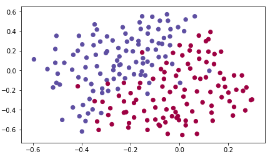
We will find where the goal keeper should kick the ball so that the French team's players can then hit it with their head. Each dot corrensponds to a position on the footbal field where a footbal player has hit the ball. The blue dot means the French player managed to hit the ball. The red dot means the other team's player hit the ball.

 

 

 

MAIN

def model(X, Y, learning_rate = 0.3, num_iterations = 30000, print_cost = True, lambd = 0, keep_prob = 1):
    """
    Implements a three-layer neural network: LINEAR->RELU->LINEAR->RELU->LINEAR->SIGMOID.
    
    Arguments:
    X -- input data, of shape (input size, number of examples)
    Y -- true "label" vector (1 for blue dot / 0 for red dot), of shape (output size, number of examples)
    learning_rate -- learning rate of the optimization
    num_iterations -- number of iterations of the optimization loop
    print_cost -- If True, print the cost every 10000 iterations
    lambd -- regularization hyperparameter, scalar
    keep_prob - probability of keeping a neuron active during drop-out, scalar.
    
    Returns:
    parameters -- parameters learned by the model. They can then be used to predict.
    """
        
    grads = {}
    costs = []                            # to keep track of the cost
    m = X.shape[1]                        # number of examples
    layers_dims = [X.shape[0], 20, 3, 1]
    
    # Initialize parameters dictionary.
    parameters = initialize_parameters(layers_dims)
 
    # Loop (gradient descent)
 
    for i in range(0, num_iterations):
 
        # Forward propagation: LINEAR -> RELU -> LINEAR -> RELU -> LINEAR -> SIGMOID.
        if keep_prob == 1:
            a3, cache = forward_propagation(X, parameters)
        elif keep_prob < 1:
            a3, cache = forward_propagation_with_dropout(X, parameters, keep_prob)
        
        # Cost function
        if lambd == 0:
            cost = compute_cost(a3, Y)
        else:
            cost = compute_cost_with_regularization(a3, Y, parameters, lambd)
            
        # Backward propagation.
        assert(lambd==0 or keep_prob==1)    # it is possible to use both L2 regularization and dropout, 
                                            # but this assignment will only explore one at a time
        if lambd == 0 and keep_prob == 1:
            grads = backward_propagation(X, Y, cache)
        elif lambd != 0:
            grads = backward_propagation_with_regularization(X, Y, cache, lambd)
        elif keep_prob < 1:
            grads = backward_propagation_with_dropout(X, Y, cache, keep_prob)
        
        # Update parameters.
        parameters = update_parameters(parameters, grads, learning_rate)
        
        # Print the loss every 10000 iterations
        if print_cost and i % 10000 == 0:
            print("Cost after iteration {}: {}".format(i, cost))
        if print_cost and i % 1000 == 0:
            costs.append(cost)
    
    # plot the cost
    plt.plot(costs)
    plt.ylabel('cost')
    plt.xlabel('iterations (x1,000)')
    plt.title("Learning rate =" + str(learning_rate))
    plt.show()
    
    return parameters
 

 

Without regularization

On the training set: Accuracy:   0.947867298578

On the test set: Accuracy:        0.915

 

This is decision boundry of the model without regularization.

The non-regularized model is obviously overfitting the training set. It is fitting noisy points.

 

 

L2 Regularization

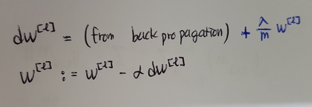
The standard way to avoid overfitting is L2 regularization. 

 

 

Implement compute_cost_with_regularization() which computes the cost given by formula above.

To calculate this, use np.sum(np.square(Wl))

 

def compute_cost_with_regularization(A3, Y, parameters, lambd):
    """
    Implement the cost function with L2 regularization. See formula (2) above.
    
    Arguments:
    A3 -- post-activation, output of forward propagation, of shape (output size, number of examples)
    Y -- "true" labels vector, of shape (output size, number of examples)
    parameters -- python dictionary containing parameters of the model
    
    Returns:
    cost - value of the regularized loss function (formula (2))
    """
    m = Y.shape[1]
    W1 = parameters["W1"]
    W2 = parameters["W2"]
    W3 = parameters["W3"]
    
    cross_entropy_cost = compute_cost(A3, Y) # This gives you the cross-entropy part of the cost
    
    ### START CODE HERE ### (approx. 1 line)
    L2_regularization_cost = 1/m * lambd/2 * (np.sum(np.square(W1)) + np.sum(np.square(W2)) + np.sum(np.square(W3)))
 
    ### END CODER HERE ###
    
    cost = cross_entropy_cost + L2_regularization_cost
    
    return cost
 

 

Because we chagned the cost, we have to change backward propagation as well.

 

def backward_propagation_with_regularization(X, Y, cache, lambd):
    """
    Implements the backward propagation of our baseline model to which we added an L2 regularization.
    
    Arguments:
    X -- input dataset, of shape (input size, number of examples)
    Y -- "true" labels vector, of shape (output size, number of examples)
    cache -- cache output from forward_propagation()
    lambd -- regularization hyperparameter, scalar
    
    Returns:
    gradients -- A dictionary with the gradients with respect to each parameter, activation and pre-activation variables
    """
    
    m = X.shape[1]
    (Z1, A1, W1, b1, Z2, A2, W2, b2, Z3, A3, W3, b3) = cache
    
    dZ3 = A3 - Y
    
    ### START CODE HERE ### (approx. 1 line)
    dW3 = 1./m * np.dot(dZ3, A2.T) + lambd/m*W3
    ### END CODE HERE ###
    db3 = 1./m * np.sum(dZ3, axis=1, keepdims = True)
    
    dA2 = np.dot(W3.T, dZ3)
    dZ2 = np.multiply(dA2, np.int64(A2 > 0))
    ### START CODE HERE ### (approx. 1 line)
    dW2 = 1./m * np.dot(dZ2, A1.T) + lambd/m*W2
    ### END CODE HERE ###
    db2 = 1./m * np.sum(dZ2, axis=1, keepdims = True)
    
    dA1 = np.dot(W2.T, dZ2)
    dZ1 = np.multiply(dA1, np.int64(A1 > 0))
    ### START CODE HERE ### (approx. 1 line)
    dW1 = 1./m * np.dot(dZ1, X.T) + lambd/m*W1
    ### END CODE HERE ###
    db1 = 1./m * np.sum(dZ1, axis=1, keepdims = True)
    
    gradients = {"dZ3": dZ3, "dW3": dW3, "db3": db3,"dA2": dA2,
                 "dZ2": dZ2, "dW2": dW2, "db2": db2, "dA1": dA1, 
                 "dZ1": dZ1, "dW1": dW1, "db1": db1}
    
    return gradients
 
 

 

Running the model with L2 regularization( lambda = 0.7 ) L2 regularization makes decision boundry smoother. If lambda is too large, it is also prossible to oversmooth, resulting in a model with high bias.

What is L2-regularization actually doing?

• L2 regularization relies on the assumption that a model with small weights is simpler than a model with large weights. Thus, by penalizing the square values of the weights in the cost function we drive all the weights to smaller values. It becomes too costly for cost to have large weights. This leads to a smoother model in which the output changes more slowly as the input changes.

 

Dropout

 

 

def backward_propagation_with_dropout(X, Y, cache, keep_prob):
    """
    Implements the backward propagation of our baseline model to which we added dropout.
    
    Arguments:
    X -- input dataset, of shape (2, number of examples)
    Y -- "true" labels vector, of shape (output size, number of examples)
    cache -- cache output from forward_propagation_with_dropout()
    keep_prob - probability of keeping a neuron active during drop-out, scalar
    
    Returns:
    gradients -- A dictionary with the gradients with respect to each parameter, activation and pre-activation variables
    """
    
    m = X.shape[1]
    (Z1, D1, A1, W1, b1, Z2, D2, A2, W2, b2, Z3, A3, W3, b3) = cache
    
    dZ3 = A3 - Y
    dW3 = 1./m * np.dot(dZ3, A2.T)
    db3 = 1./m * np.sum(dZ3, axis=1, keepdims = True)
    dA2 = np.dot(W3.T, dZ3)
    ### START CODE HERE ### (≈ 2 lines of code)
    dA2 = np.multiply(dA2, D2)              # Step 1: Apply mask D2 to shut down the same neurons as during the forward propagation
    dA2 = dA2 / keep_prob              # Step 2: Scale the value of neurons that haven't been shut down
    ### END CODE HERE ###
    dZ2 = np.multiply(dA2, np.int64(A2 > 0))
    dW2 = 1./m * np.dot(dZ2, A1.T)
    db2 = 1./m * np.sum(dZ2, axis=1, keepdims = True)
    
    dA1 = np.dot(W2.T, dZ2)
    ### START CODE HERE ### (≈ 2 lines of code)
    dA1 = np.multiply(dA1, D1)              # Step 1: Apply mask D1 to shut down the same neurons as during the forward propagation
    dA1 = dA1 / keep_prob               # Step 2: Scale the value of neurons that haven't been shut down
    ### END CODE HERE ###
    dZ1 = np.multiply(dA1, np.int64(A1 > 0))
    dW1 = 1./m * np.dot(dZ1, X.T)
    db1 = 1./m * np.sum(dZ1, axis=1, keepdims = True)
    
    gradients = {"dZ3": dZ3, "dW3": dW3, "db3": db3,"dA2": dA2,
                 "dZ2": dZ2, "dW2": dW2, "db2": db2, "dA1": dA1, 
                 "dZ1": dZ1, "dW1": dW1, "db1": db1}
    
    return gradients
 

 

Running the model with dropout( keep_prob = 0.86 ). 

Remind about dropout

• Don't use dropout during test time.
• Dropout is a regularization technique.
• Apply dropout both during forward and backward propagation.
• Divide each dropout layer by keep_prob to the same expected value for the activations. 

CONCLUSION

Regularization hurts training set performance. This is because it limits the ability of the network to overfit to the training set. But since it ultimately gives better test accuracy, it is helping our system.