This note is based on Coursera course by Andrew ng.
(It is just study note for me. It could be copied or awkward sometimes for sentence anything, because i am not native. But, i want to learn Deep Learning on English. So, everything will be bettter and better :))
INTRO
We are going to initialize the weights to separate the blue dots from the red dots.
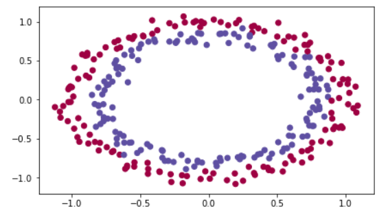
We will use a 3-layer neural network. And we will try 3 initialization.
- Zero initialization
- Random initialization
- He initialization
Neural Network model
|
1
2
3
4
5
6
7
8
9
10
11
12
13
14
15
16
17
18
19
20
21
22
23
24
25
26
27
28
29
30
31
32
33
34
35
36
37
38
39
40
41
42
43
44
45
46
47
48
49
50
51
52
53
54
55
56
57
58
|
def model(X, Y, learning_rate = 0.01, num_iterations = 15000, print_cost = True, initialization = "he"):
"""
Implements a three-layer neural network: LINEAR->RELU->LINEAR->RELU->LINEAR->SIGMOID.
Arguments:
X -- input data, of shape (2, number of examples)
Y -- true "label" vector (containing 0 for red dots; 1 for blue dots), of shape (1, number of examples)
learning_rate -- learning rate for gradient descent
num_iterations -- number of iterations to run gradient descent
print_cost -- if True, print the cost every 1000 iterations
initialization -- flag to choose which initialization to use ("zeros","random" or "he")
Returns:
parameters -- parameters learnt by the model
"""
grads = {}
costs = [] # to keep track of the loss
m = X.shape[1] # number of examples
layers_dims = [X.shape[0], 10, 5, 1]
# Initialize parameters dictionary.
if initialization == "zeros":
parameters = initialize_parameters_zeros(layers_dims)
elif initialization == "random":
parameters = initialize_parameters_random(layers_dims)
elif initialization == "he":
parameters = initialize_parameters_he(layers_dims)
# Loop (gradient descent)
for i in range(0, num_iterations):
# Forward propagation: LINEAR -> RELU -> LINEAR -> RELU -> LINEAR -> SIGMOID.
a3, cache = forward_propagation(X, parameters)
# Loss
cost = compute_loss(a3, Y)
# Backward propagation.
grads = backward_propagation(X, Y, cache)
# Update parameters.
parameters = update_parameters(parameters, grads, learning_rate)
# Print the loss every 1000 iterations
if print_cost and i % 1000 == 0:
print("Cost after iteration {}: {}".format(i, cost))
# plot the loss
plt.ylabel('cost')
plt.xlabel('iterations (per hundreds)')
return parameters
http://colorscripter.com/info#e" target="_blank" style="color:#4f4f4ftext-decoration:none">Colored by Color Scripter
|
MAIN
Zero initialization
The weight matrices (W[1], W[2], W[3], ...,W[L−1], W[L])
The bias vectors (b[1], b[2], b[3], ..., b[L−1], b[L])
|
1
2
3
4
5
6
7
8
9
10
11
12
13
14
15
16
17
18
19
20
21
22
23
|
def initialize_parameters_zeros(layers_dims):
"""
Arguments:
layer_dims -- python array (list) containing the size of each layer.
Returns:
parameters -- python dictionary containing your parameters "W1", "b1", ..., "WL", "bL":
W1 -- weight matrix of shape (layers_dims[1], layers_dims[0])
b1 -- bias vector of shape (layers_dims[1], 1)
...
WL -- weight matrix of shape (layers_dims[L], layers_dims[L-1])
bL -- bias vector of shape (layers_dims[L], 1)
"""
parameters = {}
L = len(layers_dims) # number of layers in the network
for l in range(1, L):
### START CODE HERE ### (≈ 2 lines of code)
### END CODE HERE ###
return parameters
http://colorscripter.com/info#e" target="_blank" style="color:#4f4f4ftext-decoration:none">Colored by Color Scripter
|
If we run the model with zero initialization, the performance is really bad and the cost does not really decrease, and the algorithm performs no better than random guessing. Let's look at the predictions and the decision boundry.
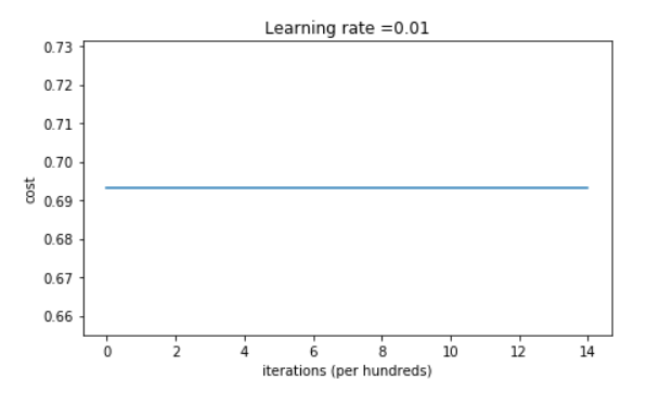
predictions_train = [[0 0 0 0 0 0 0 0 0 0 0 0 0 0 0 0 0 0 0 0 0 0 0 0 0 0 0 0 0 0 0 0 0 0 0 0 0 0 0 0 0 0 0 0 0 0 0 0 0 0 0 0 0 0 0 0 0 0 0 0 0 0 0 0 0 0 0 0 0 0 0 0 0 0 0 0 0 0 0 0 0 0 0 0 0 0 0 0 0 0 0 0 0 0 0 0 0 0 0 0 0 0 0 0 0 0 0 0 0 0 0 0 0 0 0 0 0 0 0 0 0 0 0 0 0 0 0 0 0 0 0 0 0 0 0 0 0 0 0 0 0 0 0 0 0 0 0 0 0 0 0 0 0 0 0 0 0 0 0 0 0 0 0 0 0 0 0 0 0 0 0 0 0 0 0 0 0 0 0 0 0 0 0 0 0 0 0 0 0 0 0 0 0 0 0 0 0 0 0 0 0 0 0 0 0 0 0 0 0 0 0 0 0 0 0 0 0 0 0 0 0 0 0 0 0 0 0 0 0 0 0 0 0 0 0 0 0 0 0 0 0 0 0 0 0 0 0 0 0 0 0 0 0 0 0 0 0 0 0 0 0 0 0 0 0 0 0 0 0 0 0 0 0 0 0 0 0 0 0 0 0 0 0 0 0 0 0 0 0 0 0 0 0 0 0 0 0 0 0 0]]
predictions_test = [[0 0 0 0 0 0 0 0 0 0 0 0 0 0 0 0 0 0 0 0 0 0 0 0 0 0 0 0 0 0 0 0 0 0 0 0 0 0 0 0 0 0 0 0 0 0 0 0 0 0 0 0 0 0 0 0 0 0 0 0 0 0 0 0 0 0 0 0 0 0 0 0 0 0 0 0 0 0 0 0 0 0 0 0 0 0 0 0 0 0 0 0 0 0 0 0 0 0 0 0]]
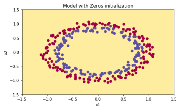
The model is predicting 0 for every example. In general, initializing all the weights to zero results in the network failing to break symmetry. This means that every neuran in each layer will learn the same thing, and we might as well as training a neural network with n[l] = 1 for every layer, and the network is no more powerful than a linear classifier such as logistic regression.
Random initialization
To break symmetry, let's initialize the weights randomly. Each neuron can then proceed to learn a different function of its inputs.
|
1
2
3
4
5
6
7
8
9
10
11
12
13
14
15
16
17
18
19
20
21
22
23
24
25
|
def initialize_parameters_random(layers_dims):
"""
Arguments:
layer_dims -- python array (list) containing the size of each layer.
Returns:
parameters -- python dictionary containing your parameters "W1", "b1", ..., "WL", "bL":
W1 -- weight matrix of shape (layers_dims[1], layers_dims[0])
b1 -- bias vector of shape (layers_dims[1], 1)
...
WL -- weight matrix of shape (layers_dims[L], layers_dims[L-1])
bL -- bias vector of shape (layers_dims[L], 1)
"""
parameters = {}
L = len(layers_dims) # integer representing the number of layers
for l in range(1, L):
### START CODE HERE ### (≈ 2 lines of code)
### END CODE HERE ###
return parameters
http://colorscripter.com/info#e" target="_blank" style="color:#4f4f4ftext-decoration:none">Colored by Color Scripter
|
If we run the following code to train model on 15,000 iterations using random initialization.
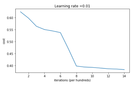
And it gives us better results.
predictions_train = [[1 0 1 1 0 0 1 1 1 1 1 0 1 0 0 1 0 1 1 0 0 0 1 0 1 1 1 1 1 1 0 1 1 0 0 1 1 1 1 1 1 1 1 0 1 1 1 1 0 1 0 1 1 1 1 0 0 1 1 1 1 0 1 1 0 1 0 1 1 1 1 0 0 0 0 0 1 0 1 0 1 1 1 0 0 1 1 1 1 1 1 0 0 1 1 1 0 1 1 0 1 0 1 1 0 1 1 0 1 0 1 1 0 0 1 0 0 1 1 0 1 1 1 0 1 0 0 1 0 1 1 1 1 1 1 1 0 1 1 0 0 1 1 0 0 0 1 0 1 0 1 0 1 1 1 0 0 1 1 1 1 0 1 1 0 1 0 1 1 0 1 0 1 1 1 1 0 1 1 1 1 0 1 0 1 0 1 1 1 1 0 1 1 0 1 1 0 1 1 0 1 0 1 1 1 0 1 1 1 0 1 0 1 0 0 1 0 1 1 0 1 1 0 1 1 0 1 1 1 0 1 1 1 1 0 1 0 0 1 1 0 1 1 1 0 0 0 1 1 0 1 1 1 1 0 1 1 0 1 1 1 0 0 1 0 0 0 1 0 0 0 1 1 1 1 0 0 0 0 1 1 1 1 0 0 1 1 1 1 1 1 1 0 0 0 1 1 1 1 0]]
predictions_test = [[1 1 1 1 0 1 0 1 1 0 1 1 1 0 0 0 0 1 0 1 0 0 1 0 1 0 1 1 1 1 1 0 0 0 0 1 0 1 1 0 0 1 1 1 1 1 0 1 1 1 0 1 0 1 1 0 1 0 1 0 1 1 1 1 1 1 1 1 1 0 1 0 1 1 1 1 1 0 1 0 0 1 0 0 0 1 1 0 1 1 0 0 0 1 1 0 1 1 0 0]]
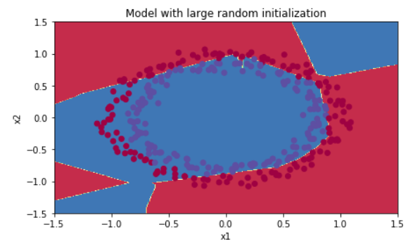
We multiply W[l] by 10. It is not much big, but if it more bigger, it can lead to exploding gradients(vanishing), which also slows down the optimization algorithm. So, initializing with small random values does better. But, how small should be these random values be? He initialization.
He initialization
This is named for the first author of He et al., 2015. This is similar except Xavier initialization uses a scaling factor for the weight W[l] of sqrt(1./layers_dims[l-1]) where He initialization would use sqrt(2./layers_dims[l-1]).
|
1
2
3
4
5
6
7
8
9
10
11
12
13
14
15
16
17
18
19
20
21
22
23
24
25
|
def initialize_parameters_he(layers_dims):
"""
Arguments:
layer_dims -- python array (list) containing the size of each layer.
Returns:
parameters -- python dictionary containing your parameters "W1", "b1", ..., "WL", "bL":
W1 -- weight matrix of shape (layers_dims[1], layers_dims[0])
b1 -- bias vector of shape (layers_dims[1], 1)
...
WL -- weight matrix of shape (layers_dims[L], layers_dims[L-1])
bL -- bias vector of shape (layers_dims[L], 1)
"""
parameters = {}
L = len(layers_dims) - 1 # integer representing the number of layers
for l in range(1, L + 1):
### START CODE HERE ### (≈ 2 lines of code)
parameters['W' + str(l)] = np.random.randn(layers_dims[l], layers_dims[l-1]) * (2./layers_dims[l-1])**0.5
### END CODE HERE ###
return parameters
http://colorscripter.com/info#e" target="_blank" style="color:#4f4f4ftext-decoration:none">Colored by Color Scripter
|
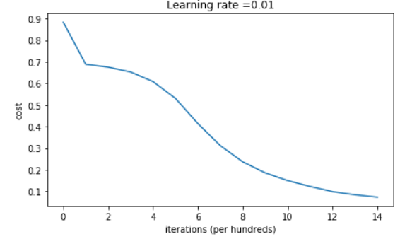
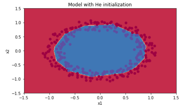
Run the following code to train model on 15,000 iterations using He initialization.
CONCLUSION

Remind!
Different initializations lead to different results.
Random initialization is used to break symmetry and make use different hidden units can learn different things.
Don't initialize to values that are too large.
He initialization works well for networks with ReLU activiations.